Specifically, the Fast Fourier Transform code further down in this tutorial only supports power-of-two sized inputs, while good libraries can do FFT on arbitrary sizes.
Here are a few good free libraries (carefully note which license they have to check if you can use it in your project):


// working with fixed sizes for simplicity in this tutorial
const int N = 128;

double fRe[N]; //the function's real part, imaginary part, and amplitude
double fIm[N];
double fAmp[N];
double FRe[N]; //the FT's real part, imaginary part and amplitude
double FIm[N];
double FAmp[N];
const double pi = 3.1415926535897932384626433832795;

void DFT(int n, bool inverse, const double *gRe, const double *gIm, double *GRe, double *GIm); //Calculates the DFT
void plot(int yPos, const double *g, double scale, bool trans, ColorRGB color); //plots a function
void calculateAmp(int n, double *ga, const double *gRe, const double *gIm); //calculates the amplitude of a complex function
|
int main(int /*argc*/, char */*argv*/[])
{
screen(640, 480, 0, "1D DFT");
cls(RGB_White);
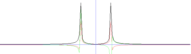
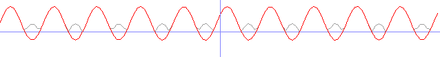
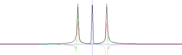
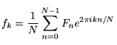
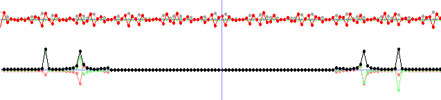
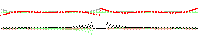
for(int x = 0; x < N; x++)
{
fRe[x] = 25 * sin(x / 2.0); //generate a sine signal. Put anything else you like here.
fIm[x] = 0;
}
//Plot the signal
calculateAmp(N, fAmp, fRe, fIm);
plot(100, fAmp, 1.0, 0, ColorRGB(160, 160, 160));
plot(100, fIm, 1.0, 0, ColorRGB(128, 255, 128));
plot(100, fRe, 1.0, 0, ColorRGB(255, 0, 0));
DFT(N, 0, fRe, fIm, FRe, FIm);
//Plot the FT of the signal
calculateAmp(N, FAmp, FRe, FIm);
plot(350, FRe, 12.0, 1, ColorRGB(255, 128, 128));
plot(350, FIm, 12.0, 1, ColorRGB(128, 255, 128));
plot(350, FAmp, 12.0, 1, ColorRGB(0, 0, 0));
drawLine(w / 2, 0, w / 2, h - 1, ColorRGB(128, 128, 255));
redraw();
sleep();
return 0;
}
|
void DFT(int n, bool inverse, const double *gRe, const double *gIm, double *GRe, double *GIm)
{
  for(int w = 0; w < n; w++)
  {
    GRe[w] = GIm[w] = 0;
    for(int x = 0; x < n; x++)
    {
      double a = -2 * pi * w * x / float(n);
      if(inverse) a = -a;
      double ca = cos(a);
      double sa = sin(a);
      GRe[w] += gRe[x] * ca - gIm[x] * sa;
      GIm[w] += gRe[x] * sa + gIm[x] * ca;
    }
    if(!inverse)
    {
      GRe[w] /= n;
      GIm[w] /= n;
    }
  }
}
|
void plot(int yPos, const double *g, double scale, bool shift, ColorRGB color)
{
  drawLine(0, yPos, w - 1, yPos, ColorRGB(128, 128, 255));
  for(int x = 1; x < N; x++)
  {
    int x1, x2, y1, y2;
    int x3, x4, y3, y4;
    x1 = (x - 1) * 5;
    //Get first endpoint, use the one half a period away if shift is used
    if(!shift) y1 = -int(scale * g[x - 1]) + yPos;
    else y1 = -int(scale * g[(x - 1 + N / 2) % N]) + yPos;
    x2 = x * 5;
    //Get next endpoint, use the one half a period away if shift is used
    if(!shift) y2 = -int(scale * g[x]) + yPos;
    else y2 = -int(scale * g[(x + N / 2) % N]) + yPos;
    //Clip the line to the screen so we won't be drawing outside the screen
    clipLine(x1, y1, x2, y2, x3, y3, x4, y4);
    drawLine(x3, y3, x4, y4, color);
    //Draw circles to show that our function is made out of discrete points
    drawDisk(x4, y4, 2, color);
  }
}
|
//Calculates the amplitude of *gRe and *gIm and puts the result in *gAmp
void calculateAmp(int n, double *gAmp, const double *gRe, const double *gIm)
{
  for(int x = 0; x < n; x++)
  {
    gAmp[x] = sqrt(gRe[x] * gRe[x] + gIm[x] * gIm[x]);
  }
}
|
There exist other algorithms that can operate fast on signals with other sizes
than a power of two, even large primes. For example mixed-radix Cooley-Tukey as well as others. However,
this is beyond the scope of this tutorial. The code linked to in the
Libraries section above supports non-powers of two so I would
recommend using a library like those for real life applications. But for this tutorial,
we continue with much simpler code for the demonstration.
Here's a new version of the DFT function, called FFT, which uses
the radix-2 algorithm described above. You
can add it to the previous program and change the function call of
it to FFT to test it out.
First, this function will calculate the logarithm of n, needed for
the algorithm.
void FFT(int n, bool inverse, const double *gRe, const double *gIm, double *GRe, double *GIm)
{
  //Calculate m=log_2(n)
  int m = 0;
  int p = 1;
  while(p < n)
  {
    p *= 2;
    m++;
  }
|
  //Bit reversal
  GRe[n - 1] = gRe[n - 1];
  GIm[n - 1] = gIm[n - 1];
  int j = 0;
  for(int i = 0; i < n - 1; i++)
  {
    GRe[i] = gRe[j];
    GIm[i] = gIm[j];
    int k = n / 2;
    while(k <= j)
    {
      j -= k;
      k /= 2;
    }
    j += k;
  }
|
  //Calculate the FFT
  double ca = -1.0;
  double sa = 0.0;
  int l1 = 1, l2 = 1;
  for(int l = 0; l < m; l++)
  {
    l1 = l2;
    l2 *= 2;
    double u1 = 1.0;
    double u2 = 0.0;
    for(int j = 0; j < l1; j++)
    {
      for(int i = j; i < n; i += l2)
      {
        int i1 = i + l1;
        double t1 = u1 * GRe[i1] - u2 * GIm[i1];
        double t2 = u1 * GIm[i1] + u2 * GRe[i1];
        GRe[i1] = GRe[i] - t1;
        GIm[i1] = GIm[i] - t2;
        GRe[i] += t1;
        GIm[i] += t2;
      }
      double z =  u1 * ca - u2 * sa;
      u2 = u1 * sa + u2 * ca;
      u1 = z;
    }
    sa = sqrt((1.0 - ca) / 2.0);
    if(!inverse) sa =- sa;
    ca = sqrt((1.0 + ca) / 2.0);
  }
|
  //Divide through n if it isn't the IDFT
  if(!inverse)
  for(int i = 0; i < n; i++)
  {
    GRe[i] /= n;
    GIm[i] /= n;
  }
}
|
const int N = 128; //yeah ok, we use old fashioned fixed size arrays here

double fRe[N]; //the function's real part, imaginary part, and amplitude
double fIm[N];
double fAmp[N];
double FRe[N]; //the FT's real part, imaginary part and amplitude
double FIm[N];
double FAmp[N];
const double pi = 3.1415926535897932384626433832795;

void FFT(int n, bool inverse, const double *gRe, const double *gIm, double *GRe, double *GIm); //Calculates the DFT
void plot(int yPos, const double *g, double scale, bool trans, ColorRGB color); //plots a function
void calculateAmp(int n, double *ga, const double *gRe, const double *gIm); //calculates the amplitude of a complex function
|
int main(int /*argc*/, char */*argv*/[])
{
screen(640, 480, 0, "Fourier Transform and Filters");
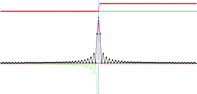
for(int x = 0; x < N; x++) fRe[x] = fIm[x] = 0;
bool endloop = 0, changed = 1;
int n = N;
double p1 = 25.0, p2 = 2.0;
while(!endloop)
{
if(done()) end();
readKeys();
|
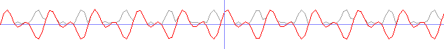
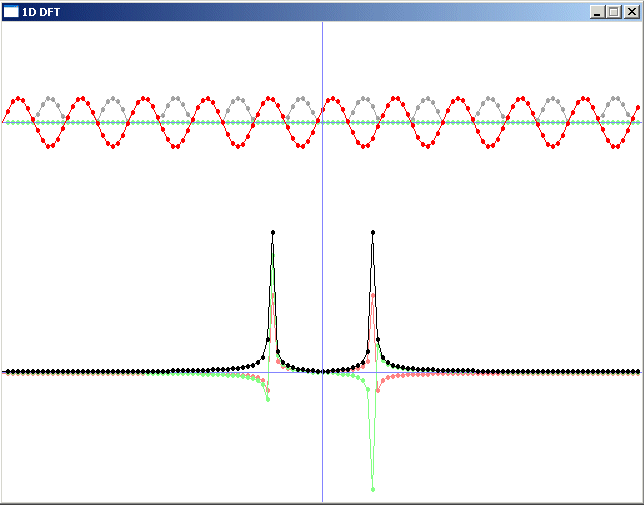
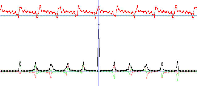
    if(keyPressed(SDLK_z)) {for(int x = 0; x < n; x++) fRe[x] = 0; changed = 1;} //zero
    if(keyPressed(SDLK_a)) {for(int x = 0; x < n; x++) fRe[x] = p1; changed = 1;} //constant
    if(keyPressed(SDLK_b)) {for(int x = 0; x < n; x++) fRe[x] = p1 * sin(x / p2); changed = 1;} //sine


    //ETCETERA... *snip*

    if(keyPressed(SDLK_SPACE)) endloop = 1;
|
    if(changed)
    {
      cls(RGB_White);
      calculateAmp(N, fAmp, fRe, fIm);
      plot(100, fAmp, 1.0, 0, ColorRGB(160, 160, 160));
      plot(100, fIm, 1.0, 0, ColorRGB(128, 255, 128));
      plot(100, fRe, 1.0, 0, ColorRGB(255, 0, 0));

      FFT(N, 0, fRe, fIm, FRe, FIm);
      calculateAmp(N, FAmp, FRe, FIm);
      plot(350, FRe, 12.0, 1, ColorRGB(255, 128, 128));
      plot(350, FIm, 12.0, 1, ColorRGB(128, 255, 128));
      plot(350, FAmp, 12.0, 1, ColorRGB(0, 0, 0));

      drawLine(w / 2, 0, w / 2, h - 1, ColorRGB(128, 128, 255));
      print("Press a-z to choose a function, press the arrows to change the imaginary part, press space to accept.", 0, 0, RGB_Black);
      redraw();
    }
    changed = 0;
  }
|
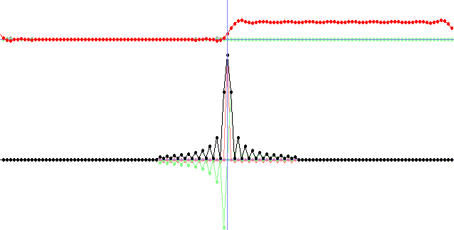
  //The original FRe2, FIm2 and FAmp2 will become multiplied by the filter
  double FRe2[N];
  double FIm2[N];
  double FAmp2[N];
  for(int x = 0; x < N; x++)
  {
    FRe2[x] = FRe[x];
    FIm2[x] = FIm[x];
  }
  cls();
  changed = 1; endloop = 0;
  while(!endloop)
  {
    if(done()) end();
    readKeys();
|
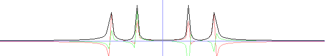
    if(keyPressed(SDLK_z))
    {
      for(int x = 0; x < n; x++)
      {
        FRe2[x] = FRe[x];
        FIm2[x] = FIm[x];
      }
      changed = 1;
    } //no filter
    if(keyPressed(SDLK_a))
    {
      for(int x = 0; x < n; x++)
      {
        if(x < 44 || x > N - 44)
        {
          FRe2[x] = FRe[x];
          FIm2[x] = FIm[x];
        }
        else FRe2[x] = FIm2[x] = 0;
      }
      changed = 1;
    } //LP

    //ETCETERA... *snip*
|
    if(changed)
    {
      cls(RGB_White);
      FFT(N, 1, FRe2, FIm2, fRe, fIm);
      calculateAmp(N, fAmp, fRe, fIm);
      plot(100, fAmp, 1.0, 0, ColorRGB(160, 160, 160));
      plot(100, fIm, 1.0, 0, ColorRGB(128, 255, 128));
      plot(100, fRe, 1.0, 0, ColorRGB(255, 0, 0));

      calculateAmp(N, FAmp2, FRe2, FIm2);

      plot(350, FRe2, 12.0, 1, ColorRGB(255, 128, 128));
      plot(350, FIm2, 12.0, 1, ColorRGB(128, 255, 128));
      plot(350, FAmp2, 12.0, 1, ColorRGB(0, 0, 0));

      drawLine(w/2, 0,w/2,h-1, ColorRGB(128, 128, 255));
      print("Press a-z to choose a filter. Press esc to quit.", 0, 0, RGB_Black);
      redraw();
    }
    changed=0;
  }

  return 0;
}
|
/// working with fixed sizes for simplicity in this tutorial
const int W = 128; //the width of the image
const int H = 128; //the height of the image

double fRe[H][W][3], fIm[H][W][3], fAmp[H][W][3]; //the signal's real part, imaginary part, and amplitude
double FRe[H][W][3], FIm[H][W][3], FAmp[H][W][3]; //the FT's real part, imaginary part and amplitude
double fRe2[H][W][3], fIm2[H][W][3], fAmp2[H][W][3]; //will become the signal again after IDFT of the spectrum
double FRe2[H][W][3], FIm2[H][W][3], FAmp2[H][W][3]; //filtered spectrum

double pi = 3.1415926535897932384626433832795;

void draw(int xpos, int yPos, int w, int h, const double *g, bool shift, bool neg128);
void DFT2D(int w, int h, bool inverse, const double *gRe, const double *gIm, double *GRe, double *GIm);
void FFT2D(int w, int h, bool inverse, const double *gRe, const double *gIm, double *GRe, double *GIm);
void calculateAmp(int w, int h, double *ga, const double *gRe, const double *gIm);
|
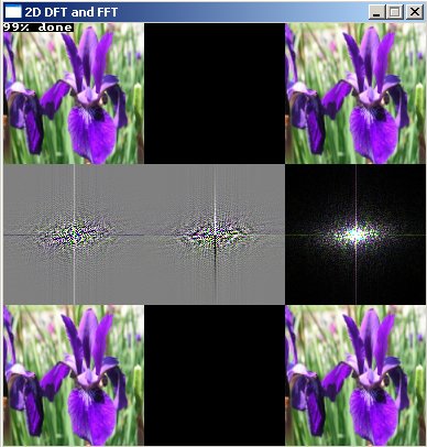
int main(int /*argc*/, char */*argv*/[])
{
screen(N * 3, M * 3, 0, "2D DFT and FFT");
std::vector<ColorRGB> img;
unsigned long dummyw, dummyh;
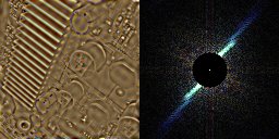
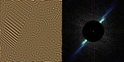
if(loadImage(img, dummyw, dummyh, "pics/test.png"))
{
print("image pics/test.png not found");
redraw();
sleep();
cls();
}
//set signal to the image
for(int y = 0; y < H; y++)
for(int x = 0; x < W; x++)
{
fRe[y][x][0] = img[W * y + x].r;
fRe[y][x][1] = img[W * y + x].g;
fRe[y][x][2] = img[W * y + x].b;
}
//draw the image (real, imaginary and amplitude)
calculateAmp(W, H, fAmp[0][0], fRe[0][0], fIm[0][0]);
draw(0, 0, W, H, fRe[0][0], 0, 0);
draw(W, 0, W, H, fIm[0][0], 0, 0);
draw(2 * W, 0, W, H, fAmp[0][0], 0, 0);
//calculate and draw the FT of the image
DFT2D(W, H, 0, fRe[0][0], fIm[0][0], FRe[0][0], FIm[0][0]); //Change this to FFT2D to make it faster
calculateAmp(W, H, FAmp[0][0], FRe[0][0], FIm[0][0]);
draw(0, H, W, H, FRe[0][0], 1, 1);
draw(W, H, W, H, FIm[0][0], 1, 1);
draw(2 * W, H, W, H, FAmp[0][0], 1, 0);
//calculate and draw the image again
DFT2D(W, H, 1, FRe[0][0], FIm[0][0], fRe2[0][0], fIm2[0][0]); //Change this to FFT2D to make it faster
calculateAmp(W, H, fAmp2[0][0], fRe2[0][0], fIm2[0][0]);
draw(0, 2 * H, W, H, fRe2[0][0], 0, 0);
draw(W, 2 * H, W, H, fIm2[0][0], 0, 0);
draw(2 * W, 2 * H, W, H, fAmp2[0][0], 0, 0);
redraw();
sleep();
return 0;
}
|
void DFT(int n, bool inverse, const double *gRe, const double *gIm, double *GRe, double *GIm, int stride, double factor)
{
  for(int n = 0; n < n; n++)
  {
    GRe[n * stride] = GIm[n * stride] = 0;
    for(int x = 0; x < n; x++)
    {
      double a = -2 * pi * n * x / float(n);
      if(inverse) a = -a;
      double ca = cos(a);
      double sa = sin(a);
      GRe[n * stride] += gRe[x * stride] * ca - gIm[x * stride] * sa;
      GIm[n * stride] += gRe[x * stride] * sa + gIm[x * stride] * ca;
    }
    //Divide through the factor, e.g. n
    GRe[n * stride] /= factor;
    GIm[n * stride] /= factor;
  }
}
|
void DFT2D(int w, int h, bool inverse, const double *gRe, const double *gIm, double *GRe, double *GIm)
{
  //temporary buffers
  std::vector<double> Gr2(m * n * 3);
  std::vector<double> Gi2(m * n * 3);

  for(int y = 0; y < h; y++) // for each row
  for(int c = 0; c < 3; c++) // for each color channel
  {
    DFT(w, inverse, &gRe[y * w * 3 + c], &gIm[y * w * 3 + c], &Gr2[y * w * 3 + c], &Gi2[y * w * 3 + c], 3, 1);
  }
  for(int x = 0; x < w; x++) // for each column
  for(int c = 0; c < 3; c++) // for each color channel
  {
    DFT(h, inverse, &Gr2[x * 3 + c], &Gi2[x * 3 + c], &GRe[x * 3 + c], &GIm[x * 3 + c], w * 3, inverse ? w : h);
  }
}
|
void FFT(int n, bool inverse, const double *gRe, const double *gIm, double *GRe, double *GIm, int stride, double factor)
{
  //Calculate h=log_2(n)
  int h = 0;
  int p = 1;
  while(p < n)
  {
    p *= 2;
    h++;
  }
  //Bit reversal
  GRe[(n - 1) * stride] = gRe[(n - 1) * stride];
  GIm[(n - 1) * stride] = gIm[(n - 1) * stride];
  int j = 0;
  for(int i = 0; i < n - 1; i++)
  {
    GRe[i * stride] = gRe[j * stride];
    GIm[i * stride] = gIm[j * stride];
    int k = n / 2;
    while(k <= j)
    {
      j -= k;
      k /= 2;
    }
    j += k;
  }
  //Calculate the FFT
  double ca = -1.0;
  double sa = 0.0;
  int l1 = 1, l2 = 1;
  for(int l = 0; l < h; l++)
  {
    l1 = l2;
    l2 *= 2;
    double u1 = 1.0;
    double u2 = 0.0;
    for(int j = 0; j < l1; j++)
    {
      for(int i = j; i < n; i += l2)
      {
        int i1 = i + l1;
        double t1 = u1 * GRe[i1 * stride] - u2 * GIm[i1 * stride];
        double t2 = u1 * GIm[i1 * stride] + u2 * GRe[i1 * stride];
        GRe[i1 * stride] = GRe[i * stride] - t1;
        GIm[i1 * stride] = GIm[i * stride] - t2;
        GRe[i * stride] += t1;
        GIm[i * stride] += t2;
      }
      double z =  u1 * ca - u2 * sa;
      u2 = u1 * sa + u2 * ca;
      u1 = z;
    }
    sa = sqrt((1.0 - ca) / 2.0);
    if(!inverse) sa =- sa;
    ca = sqrt((1.0 + ca) / 2.0);
  }
  //Divide through the factor, e.g. n
  for(int i = 0; i < n; i++)
  {
    GRe[i * stride] /= factor;
    GIm[i * stride] /= factor;
  }
}
|
void FFT2D(int w, int h, bool inverse, const double *gRe, const double *gIm, double *GRe, double *GIm)
{
  //temporary buffers
  std::vector<double> Gr2(m * n * 3);
  std::vector<double> Gi2(m * n * 3);

  for(int y = 0; y < h; y++) // for each row
  for(int c = 0; c < 3; c++) // for each color channel
  {
    FFT(w, inverse, &gRe[y * w * 3 + c], &gIm[y * w * 3 + c], &Gr2[y * w * 3 + c], &Gi2[y * w * 3 + c], 3, 1);
  }
  for(int x = 0; x < w; x++) // for each column
  for(int c = 0; c < 3; c++) // for each color channel
  {
    FFT(h, inverse, &Gr2[x * 3 + c], &Gi2[x * 3 + c], &GRe[x * 3 + c], &GIm[x * 3 + c], w * 3, inverse ? w : h);
  }
}
|
//Draws an image
void draw(int xPos, int yPos, int n, int m, const double *g, bool shift, bool neg128) //g is the image to be drawn
{
  for(int y = 0; y < m; y++)
  for(int x = 0; x < n; x++)
  {
    int x2 = x, y2 = y;
    if(shift) {x2 = (x + n / 2) % n; y2 = (y + m / 2) % m;} //Shift corners to center
    ColorRGB color;
    //calculate color values out of the floating point buffer
    color.r = int(g[3 * w * y2 + 3 * x2 + 0]);
    color.g = int(g[3 * w * y2 + 3 * x2 + 1]);
    color.b = int(g[3 * w * y2 + 3 * x2 + 2]);

    if(neg128) color = color + RGB_Gray;
    //negative colors give confusing effects so set them to 0
    if(color.r < 0) color.r = 0;
    if(color.g < 0) color.g = 0;
    if(color.b < 0) color.b = 0;
    //set color components higher than 255 to 255
    if(color.r > 255) color.r = 255;
    if(color.g > 255) color.g = 255;
    if(color.b > 255) color.b = 255;
    //plot the pixel
    pset(x + xPos, y + yPos, color);
  }
}
|
//Calculates the amplitude of *gRe and *gIm and puts the result in *gAmp
void calculateAmp(int n, int m, double *gAmp, const double *gRe, const double *gIm)
{
  for(int y = 0; y < m; y++)
  for(int x = 0; x < n; x++)
  for(int c = 0; c < 3; c++)
  {
    gAmp[w * 3 * y + 3 * x + c] = sqrt(gRe[w * 3 * y + 3 * x + c] * gRe[w * 3 * y + 3 * x + c] + gIm[w * 3 * y + 3 * x + c] * gIm[w * 3 * y + 3 * x + c]);
  }
}
|


// working with fixed sizes for simplicity in this tutorial
const int W = 128; //the width of the image
const int H = 128; //the height of the image

double fRe[H][W][3], fIm[H][W][3], fAmp[H][W][3]; //the signal's real part, imaginary part, and amplitude
double FRe[H][W][3], FIm[H][W][3], FAmp[H][W][3]; //the FT's real part, imaginary part and amplitude
double fRe2[H][W][3], fIm2[H][W][3], fAmp2[H][W][3]; //will become the signal again after IDFT of the spectrum
double FRe2[H][W][3], FIm2[H][W][3], FAmp2[H][W][3]; //filtered spectrum

double pi = 3.1415926535897932384626433832795;

void draw(int xpos, int yPos, int w, int h, const double *g, bool shift, bool neg128);
void DFT2D(int w, int h, bool inverse, const double *gRe, const double *gIm, double *GRe, double *GIm);
void FFT2D(int w, int h, bool inverse, const double *gRe, const double *gIm, double *GRe, double *GIm);
void calculateAmp(int w, int h, double *ga, const double *gRe, const double *gIm);
|
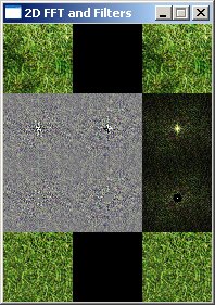
int main(int /*argc*/, char */*argv*/[])
{
screen(3 * W,4 * H + 8, 0,"2D FFT and Filters");
std::vector
|
    if(keyPressed(SDLK_z) || changed)
    {
      for(int y = 0; y < H; y++)
      for(int x = 0; x < W; x++)
      for(int c = 0; c < 3; c++)
      {
        fRe2[y][x][c] = fRe[y][x][c];
      } changed = 1;
    } //no effect
    if(keyPressed(SDLK_a))
    {
      for(int y = 0; y < H; y++)
      for(int x = 0; x < W; x++)
      for(int c = 0; c < 3; c++)
      {
        fRe2[y][x][c] = 255 - fRe[y][x][c];
      }
    changed = 1;} //negative
    if(keyPressed(SDLK_b))
    {
      for(int y = 0; y < H; y++)
      for(int x = 0; x < W; x++)
      for(int c = 0; c < 3; c++)
      {
        fRe2[y][x][c] = fRe[y][x][c]/2;
      }
      changed = 1;
    } //half amplitude


    //ETCETERA... *snip*

    if(keyPressed(SDLK_SPACE)) endloop = 1;
|
    if(changed)
    {
      //Draw the image and its FT
      calculateAmp(W, H, fAmp2[0][0], fRe2[0][0], fIm2[0][0]);
      draw(0, ytrans, W, H, fRe2[0][0], 0, 0);  draw(W, 0+ytrans, W, H, fIm2[0][0], 0, 0);  draw(2 * W, 0+ytrans, W, H, fAmp2[0][0], 0, 0); //draw real, imag and amplitude
      FFT2D(W, H, 0, fRe2[0][0], fIm2[0][0], FRe[0][0], FIm[0][0]);
      calculateAmp(W, H, FAmp[0][0], FRe[0][0], FIm[0][0]);
      draw(0,H + ytrans, W, H, FRe[0][0], 1, 1);  draw(W, H + ytrans, W, H, FIm[0][0], 1, 1);  draw(2 * W, H + ytrans, W, H, FAmp[0][0], 1, 0); //draw real, imag and amplitude
      print("Press a-z for effects and space to accept", 0, 0, RGB_White, 1, ColorRGB(128, 0, 0));
      redraw();
    }
    changed = 0;
  }
  changed = 1;
  while(!done())
  {
    readKeys();
|
    if(keyPressed(SDLK_g))
    {
      for(int y = 0; y < H; y++)
      for(int x = 0; x < W; x++)
      for(int c = 0; c < 3; c++)
      {
        if(x * x + y * y < 64 || (W - x) * (W - x) + (H - y) * (H - y) < 64 || x * x + (H - y) * (H - y) < 64 || (W - x) * (W - x) + y * y < 64)
        {
          FRe2[y][x][c] = FRe[y][x][c];
          FIm2[y][x][c] = FIm[y][x][c];
        }
        else
        {
          FRe2[y][x][c] = 0;
          FIm2[y][x][c] = 0;
        }
      }
      changed = 1;
    } //LP filter

    if(keyPressed(SDLK_h))
    {
      for(int y = 0; y < H; y++)
      for(int x = 0; x < W; x++)
      for(int c = 0; c < 3; c++)
      {
        if(x * x + y * y > 16 && (W - x) * (W - x) + (H - y) * (H - y) > 16 && x * x + (H - y) * (H - y) > 16 && (W - x) * (W - x) + y * y > 16)
        {
          FRe2[y][x][c] = FRe[y][x][c];
          FIm2[y][x][c] = FIm[y][x][c];
        }
        else
        {
          FRe2[y][x][c] = 0;
          FIm2[y][x][c] = 0;
        }
      }
      changed = 1;
    } //HP filter

    if(keyPressed(SDLK_t))
    {
      for(int y = 0; y < H; y++)
      for(int x = 0; x < W; x++)
      for(int c = 0; c < 3; c++)
      {
        if((x * x + y * y < 256 || (W - x) * (W - x) + (H - y) * (H - y) < 256 || x * x + (H - y) * (H - y) < 256 || (W - x) * (W - x) + y * y < 256) && (x * x + y * y > 128 && (W - x) * (W - x) + (H - y) * (H - y) > 128 && x * x + (H - y) * (H - y) > 128 && (W - x) * (W - x) + y * y > 128))
        {
          FRe2[y][x][c] = FRe[y][x][c];
          FIm2[y][x][c] = FIm[y][x][c];
        }
        else
        {
          FRe2[y][x][c] = 0;
          FIm2[y][x][c] = 0;
        }
      }
      changed = 1;
    } //BP filter

    //ETCETERA... *snip*
|
    if(changed)
    {
      //after pressing a key: calculate the inverse!
      FFT2D(W, H, 1, FRe2[0][0], FIm2[0][0], fRe[0][0], fIm[0][0]);
      calculateAmp(W, H, fAmp[0][0], fRe[0][0], fIm[0][0]);
      draw(0, 3 * H + ytrans, W, H, fRe[0][0], 0, 0);  draw(W, 3 * H + ytrans, W, H, fIm[0][0], 0, 0);  draw(2 * W, 3 * H + ytrans, W, H, fAmp[0][0], 0, 0);
      calculateAmp(W, H, FAmp2[0][0], FRe2[0][0], FIm2[0][0]);
      draw(0, 2 * H + ytrans, W, H, FRe2[0][0], 1, 1);  draw(W, 2 * H + ytrans, W, H, FIm2[0][0], 1, 1);  draw(2 * W, 2 * H + ytrans, W, H, FAmp2[0][0], 1, 0);
      print("Press a-z for filters and arrows to change DC", 0, 0, RGB_White, 1, ColorRGB(128, 0, 0));
      redraw();
    }
    changed=0;
  }
  return 0;
}
|
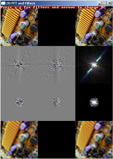
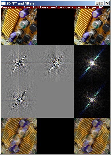

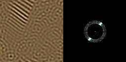
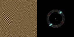
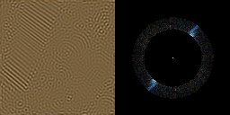
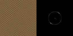
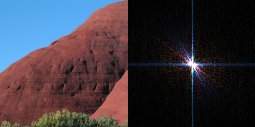
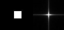
You can also, for example, keep a square one, but round ones should
give nicer blurs:
Side note: for some types of blur, such as gaussian blur, there are still other faster algorithms that don't require the FFT nor a large kernel, in the case of gaussian blur you can approximate it very well by doing three box blurs that take linear time for any size of box in a row, see the Filtering tutorial of this series for a bit more on that.

Side note: For sharpening, too, there are even faster algorithms than with FFT, such as using fast blur and then computing the following sum of images: original + (original - blur) * amount. This is "unsharp masking"