#define filterWidth 3
#define filterHeight 3
double filter[filterHeight][filterWidth] =
{
0, 0, 0,
0, 1, 0,
0, 0, 0
};
double factor = 1.0;
double bias = 0.0;
int main(int argc, char *argv[])
{
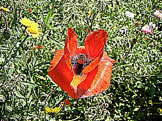
//load the image into the buffer
unsigned long w = 0, h = 0;
std::vector<ColorRGB> image;
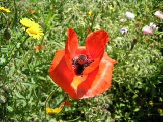
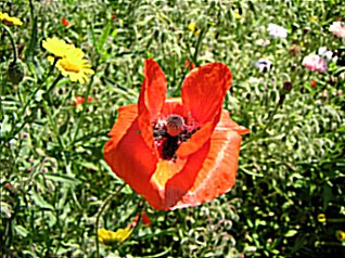
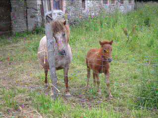
loadImage(image, w, h, "pics/photo3.png");
std::vector<ColorRGB> result(image.size());
//set up the screen
screen(w, h, 0, "Filters");
ColorRGB color; //the color for the pixels
//apply the filter
for(int x = 0; x < w; x++)
for(int y = 0; y < h; y++)
{
double red = 0.0, green = 0.0, blue = 0.0;
//multiply every value of the filter with corresponding image pixel
for(int filterY = 0; filterY < filterHeight; filterY++)
for(int filterX = 0; filterX < filterWidth; filterX++)
{
int imageX = (x - filterWidth / 2 + filterX + w) % w;
int imageY = (y - filterHeight / 2 + filterY + h) % h;
red += image[imageY * w + imageX].r * filter[filterY][filterX];
green += image[imageY * w + imageX].g * filter[filterY][filterX];
blue += image[imageY * w + imageX].b * filter[filterY][filterX];
}
//truncate values smaller than zero and larger than 255
result[y * w + x].r = min(max(int(factor * red + bias), 0), 255);
result[y * w + x].g = min(max(int(factor * green + bias), 0), 255);
result[y * w + x].b = min(max(int(factor * blue + bias), 0), 255);
}
//draw the result buffer to the screen
for(int y = 0; y < h; y++)
for(int x = 0; x < w; x++)
{
pset(x, y, result[y * w + x]);
}
//redraw & sleep
redraw();
sleep();
}
|
    //take absolute value and truncate to 255
    result[y * w + x].r = min(abs(int(factor * red + bias)), 255);
    result[y * w + x].g = min(abs(int(factor * green + bias)), 255);
    result[y * w + x].b = min(abs(int(factor * blue + bias)), 255);
|
#define filterWidth 3
#define filterHeight 3
double filter[filterHeight][filterWidth] =
{
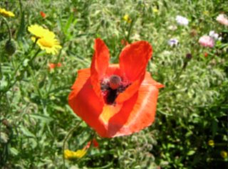
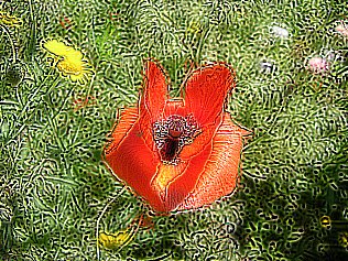
0.0, 0.2, 0.0,
0.2, 0.2, 0.2,
0.0, 0.2, 0.0
};
double factor = 1.0;
double bias = 0.0;
|
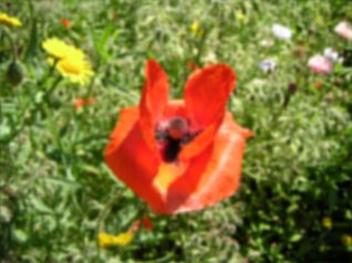
#define filterWidth 5
#define filterHeight 5

double filter[filterHeight][filterWidth] =
{
  0, 0, 1, 0, 0,
  0, 1, 1, 1, 0,
  1, 1, 1, 1, 1,
  0, 1, 1, 1, 0,
  0, 0, 1, 0, 0,
};

double factor = 1.0 / 13.0;
double bias = 0.0;
|
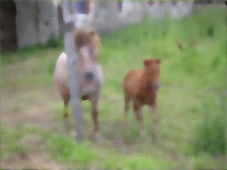
If your kernel is an entire box filled with the same value (with appropriate scaling factor so all elements sum to 1.0), then the blur is called a box blur. If you want a very large box blur, then the naive convolution code in this tutorial is too slow. But you can implement it easily with a much faster algorithm: Since every value has the same factor, you can go loop through the pixels of the image line by line, and sum N values (with N the width of the box) and divide through the appropriate scaling factor. Then for every next pixel, you add the value of the next pixel that appears in the box, and subtract the value from the leftmost pixel that disappears from the box. After doing this for each scanline horizontally, do the same vertically (to optimize use of the CPU cache, when doing it vertically, ensure that you still implement it in such way that you still operate in scanline order in practice rather than per columns, so store a sum per column). This all requires care with how you treat the edges (where the box is partially out of bounds) and the case where the image is smaller than the box. No code is given here as it goes a bit beyond the scope of this tutorial.
For 2D, you apply this formula in the X direction, then in the Y direction (it is separable), or combined it gives: G(x, y) = exp(-(x * x + y * y) / (2 * sigma * sigma)) / (2 * pi * sigma * sigma)
In the formulas:
*) sigma determines the radius (in theory the radius is in finite, but in practice due to the exponential backoff
there is a point where it becomes too small to see, the larger sigma is the further away this is)
*) x and y must be coordinates such that 0 is in the center of the kernel
The above formula tells hwo to make arbitrarily large kernels. However, here are simple examples that can be used immediately:
Approximation to 3x3 kernel:
#define filterWidth 3 #define filterHeight 3 double filter[filterHeight][filterWidth] = { 1, 2, 1, 2, 4, 2, 1, 2, 1, }; double factor = 1.0 / 16.0; double bias = 0.0;
Approximation to 5x5 kernel:
#define filterWidth 5 #define filterHeight 5 double filter[filterHeight][filterWidth] = { 1, 4, 6, 4, 1, 4, 16, 24, 16, 4, 6, 24, 36, 24, 6, 4, 16, 24, 16, 4, 1, 4, 6, 4, 1, }; double factor = 1.0 / 256.0; double bias = 0.0;
An exact intead of approximate example:
#define filterWidth 3 #define filterHeight 3 double filter[filterHeight][filterWidth] = { 0.077847, 0.123317, 0.077847, 0.123317, 0.195346, 0.123317, 0.077847, 0.123317, 0.077847, }; double factor = 1.0; double bias = 0.0;
For larger radius (such as you can try in a painting program that has gaussian blur), you need larger kernels. The naive convolution implementation like used in this tutorial would become too slow in practice for large radius gaussian blurs. But there are solutions to that: using the Fourier Transform as described in the Fourier Transform tutorial of this series, or an even faster approximation: The fast approximation involves doing multiple box blurs in a row, three in a row approximated it already very well. How to do a fast box blur is explained in the previous chapter. The reason this works is that a gaussian distribution arises naturally from a sum of other processes.
#define filterWidth 9
#define filterHeight 9

double filter[filterHeight][filterWidth] =
{
  1, 0, 0, 0, 0, 0, 0, 0, 0,
  0, 1, 0, 0, 0, 0, 0, 0, 0,
  0, 0, 1, 0, 0, 0, 0, 0, 0,
  0, 0, 0, 1, 0, 0, 0, 0, 0,
  0, 0, 0, 0, 1, 0, 0, 0, 0,
  0, 0, 0, 0, 0, 1, 0, 0, 0,
  0, 0, 0, 0, 0, 0, 1, 0, 0,
  0, 0, 0, 0, 0, 0, 0, 1, 0,
  0, 0, 0, 0, 0, 0, 0, 0, 1,
};

double factor = 1.0 / 9.0;
double bias = 0.0;
|

#define filterWidth 5
#define filterHeight 5
double filter[filterHeight][filterWidth] =
{
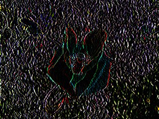
0, 0, -1, 0, 0,
0, 0, -1, 0, 0,
0, 0, 2, 0, 0,
0, 0, 0, 0, 0,
0, 0, 0, 0, 0,
};
double factor = 1.0;
double bias = 0.0;
|
#define filterWidth 5
#define filterHeight 5

double filter[filterHeight][filterWidth] =
{
   0,  0, -1,  0,  0,
   0,  0, -1,  0,  0,
   0,  0,  4,  0,  0,
   0,  0, -1,  0,  0,
   0,  0, -1,  0,  0,
};

double factor = 1.0;
double bias = 0.0;
|
#define filterWidth 5
#define filterHeight 5
double filter[filterHeight][filterWidth] =
{
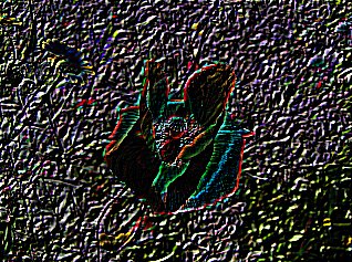
-1, 0, 0, 0, 0,
0, -2, 0, 0, 0,
0, 0, 6, 0, 0,
0, 0, 0, -2, 0,
0, 0, 0, 0, -1,
};
double factor = 1.0;
double bias = 0.0;
|
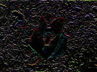
#define filterWidth 3
#define filterHeight 3
double filter[filterHeight][filterWidth] =
{
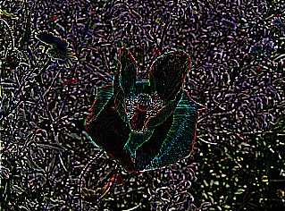
-1, -1, -1,
-1, 8, -1,
-1, -1, -1
};
double factor = 1.0;
double bias = 0.0;
|
#define filterWidth 3
#define filterHeight 3

double filter[filterHeight][filterWidth] =
{
  -1, -1, -1,
  -1,  9, -1,
  -1, -1, -1
};

double factor = 1.0;
double bias = 0.0;
|
#define filterWidth 5
#define filterHeight 5

double filter[filterHeight][filterWidth] =
{
  -1, -1, -1, -1, -1,
  -1,  2,  2,  2, -1,
  -1,  2,  8,  2, -1,
  -1,  2,  2,  2, -1,
  -1, -1, -1, -1, -1,
};

double factor = 1.0 / 8.0;
double bias = 0.0;
|
#define filterWidth 3
#define filterHeight 3

double filter[filterHeight][filterWidth] =
{
   1,  1,  1,
   1, -7,  1,
   1,  1,  1
};

double factor = 1.0;
double bias = 0.0;
|
#define filterWidth 3
#define filterHeight 3
double filter[filterHeight][filterWidth] =
{
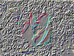
-1, -1, 0,
-1, 0, 1,
0, 1, 1
};
double factor = 1.0;
double bias = 128.0;
|
#define filterWidth 5
#define filterHeight 5
double filter[filterHeight][filterWidth] =
{
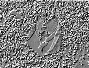
-1, -1, -1, -1, 0,
-1, -1, -1, 0, 1,
-1, -1, 0, 1, 1,
-1, 0, 1, 1, 1,
0, 1, 1, 1, 1
};
double factor = 1.0;
double bias = 128.0;
|
#define filterWidth 3
#define filterHeight 3

double filter[filterHeight][filterWidth] =
{
  1, 1, 1,
  1, 1, 1,
  1, 1, 1
};

double factor = 1.0 / 9.0;
double bias = 0.0;
|
#define filterWidth 3
#define filterHeight 3
//color arrays
int red[filterWidth * filterHeight];
int green[filterWidth * filterHeight];
int blue[filterWidth * filterHeight];
int selectKth(int* data, int s, int e, int k);
int main(int argc, char *argv[])
{
//load the image into the buffer
unsigned long w = 0, h = 0;
std::vector<ColorRGB> image;
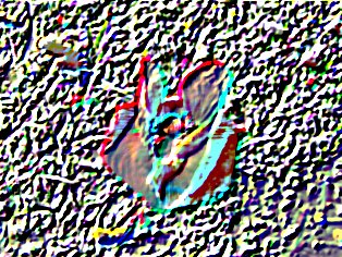
loadImage(image, w, h, "pics/noise.png");
std::vector<ColorRGB> result(image.size());
//set up the screen
screen(w, h, 0, "Median Filter");
ColorRGB color; //the color for the pixels
//apply the filter
for(int y = 0; y < h; y++)
for(int x = 0; x < w; x++)
{
int n = 0;
//set the color values in the arrays
for(int filterY = 0; filterY < filterHeight; filterY++)
for(int filterX = 0; filterX < filterWidth; filterX++)
{
int imageX = (x - filterWidth / 2 + filterX + w) % w;
int imageY = (y - filterHeight / 2 + filterY + h) % h;
red[n] = image[imageY * w + imageX].r;
green[n] = image[imageY * w + imageX].g;
blue[n] = image[imageY * w + imageX].b;
n++;
}
int filterSize = filterWidth * filterHeight;
result[y * w + x].r = red[selectKth(red, 0, filterSize, filterSize / 2)];
result[y * w + x].g = green[selectKth(green, 0, filterSize, filterSize / 2)];
result[y * w + x].b = blue[selectKth(blue, 0, filterSize, filterSize / 2)];
}
//draw the result buffer to the screen
for(int y = 0; y < h; y++)
for(int x = 0; x < w; x++)
{
pset(x, y, result[y * w + x]);
}
//redraw & sleep
redraw();
sleep();
}
|
// selects the k-th largest element from the data between start and end (end exclusive)
int selectKth(int* data, int s, int e, int k)  // in practice, use C++'s nth_element, this is for demonstration only
{
  // 5 or less elements: do a small insertion sort
  if(e - s <= 5)
  {
    for(int i = s + 1; i < e; i++)
      for(int j = i; j > 0 && data[j - 1] > data[j]; j--) std::swap(data[j], data[j - 1]);
    return s + k;
  }

  int p = (s + e) / 2; // choose simply center element as pivot

  // partition around pivot into smaller and larger elements
  std::swap(data[p], data[e - 1]); // temporarily move pivot to the end
  int j = s;  // new pivot location to be calculated
  for(int i = s; i + 1 < e; i++)
    if(data[i] < data[e - 1]) std::swap(data[i], data[j++]);
  std::swap(data[j], data[e - 1]);

  // recurse into the applicable partition
  if(k == j - s) return s + k;
  else if(k < j - s) return selectKth(data, s, j, k);
  else return selectKth(data, j + 1, e, k - j + s - 1); // subtract amount of smaller elements from k
}
|


Side note: The median algorithm implementation above is very slow. Whether using C++'s nth_element function or the toy "selectKth" here, both provide little benefit for a median of 9 or 25 numbers. No matter what the theoretical complexity of the algorithm on large N is, if you only operate on a certain small finite sized input, you need to take what works best for that input size.
If you want to implement, say, median with 3x3, then you get the fastest solution by using a hardcoded sorting network of size 9 of which you take the middle output to get the median. Then apply this for every output pixel to the corresponding 9 input pixels, and this all per color channel. The advantage of hardcoded is that the algorithm does not need to contain conditionals that depend on the size of the input (conditionals, like ifs and the for loop conditions, are very slow for CPUs as they interrupt the pipeline). No code is provided here since an efficiant practical implementation is beyond the scope of this tutorial. If interested, look up sorting network, it is a hardcoded series of swaps of two numbers depending on which is the maximum, find one that is proven to be optimal for the desired input size. Then since we don't want to fully sort but only take the median element, you can leave out every swap that does not contribute to the middle element output, and replace any swap of which only one output contributes to the middle output element with either min or max. That will give the theoretically fastest possible implementation, speedups on top of that can only be to make use of parallelism and/or better CPU instructions.